Simple Electron Microscopy Primer
The reference model obtained in the previous step is often further refined to increase the visible detail. A common method for refinement has been termed projection matching or angular refinement. This iterative process is used to better define the angular position of each experimental projection.
In random conical tilt, images were assigned angular positions through rotational alignment and tilt-angles. As described earlier, particles are first classified according to their orientation on the carbon film. From each different class, a three-dimensional preliminary model is constructed. To improve the output, those preliminary models from each class that have a high degree of similarity are merged. In theory, these models corresponded to groups of the same molecule just viewed from different orientations. If a model does not sufficiently match the other models, it is discarded.
Once all the good random conical tilt models (and their corresponding particle data sets) have been merged, iterative angular refinement is used to improve the model's resolution. Equidistant projections are first generated from the merged model. A good angular separation distance used for the first run is 15°. In this case, 89 reference projections are generated that cover the entire Euler sphere. The entire particle data set (whether the old random conical tilt experimental particles, or new untilted experimental particles, or both) is then cross correlated to each reference projection. A correlation coefficient is generated between each experimental particle and reference projection. For each individual experimental particle, it is matched to the reference projection that gave the highest correlation coefficient. Therefore, it is assumed that this particle matches the Euler angles (θ, φ, ψ) of the reference projection.

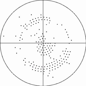
Figure 1 is an angular distribution plot showing the spread of particles in angular space around the reference model. The θ and φ axes are indicated. Each mark inside the circle indicates the position of a matched projection. The dataset that generated this distribution plot consisted only of one class of particles and their corresponding tilt pairs. The cluster of dots near the center corresponds to the untilted particles, while the surrounding ring represents the tilted particles. Ideally, one would want the distribution plot to be completely filled, indicating that all possible views of the specimen have been imaged.
Now that each experimental projection has been matched with three Euler angles, a new model is generated via back projection. Reference projections are again generated from this model (though usually at a tighter angular distance such as 5°). Experimental particles are matched to the new reference projections and a new model is generated. This procedure is repeated until the reconstructed model does not improve during iterations.
TO BE CONTINUED
Not Yet Implemented